Analysing Lens Performance
Background
Typically, when a manufacturer produces new lenses, they include an MTF chart to demonstrate the lens’s performance – sharpness measured as the number of line-pairs per millimetre it can resolve (to a given contrast tolerance), radially and sagitally, varying with distance from the centre of the image. While this might be useful before purchasing a lens, it does not make for easy comparisons (what if another manufacturer uses a different contrast tolerance?) nor does it necessarily well reflect the use to which it’ll be put in practice. (What if they quote a zoom’s performance at 28mm and 70mm f/5.6, but you shoot it most at 35mm f/8? Is the difference between radial and sagittal sharpness useful for a real-world scene?)
Further, if your lens has been around in the kit-bag a bit, is its performance still up to scratch or has it gone soft, with internal elements slightly out of alignment? When you’re out in the field, does it matter whether you use 50mm in the middle of a zoom or a fixed focal-length prime 50mm instead?
If you’re shooting landscape, would it be better to hand-hold at f/5.6 or stop-down to f/16 for depth of field, use a tripod and risk losing sharpness to diffraction?
Does that blob of dust on the front element really make a difference?
How bad is the vignetting when used wide-open?
Here’s a fairly quick experiment to measure and compare lenses’ performance by aperture, two ways. First, we design a test-chart. It’s most useful if the pattern is even across the frame, reflecting a mixture of scales of detail – thick and thin lines – at a variety of angles – at least perpendicular and maybe crazy pseudo-random designs. Here’s a couple of ideas:
Method
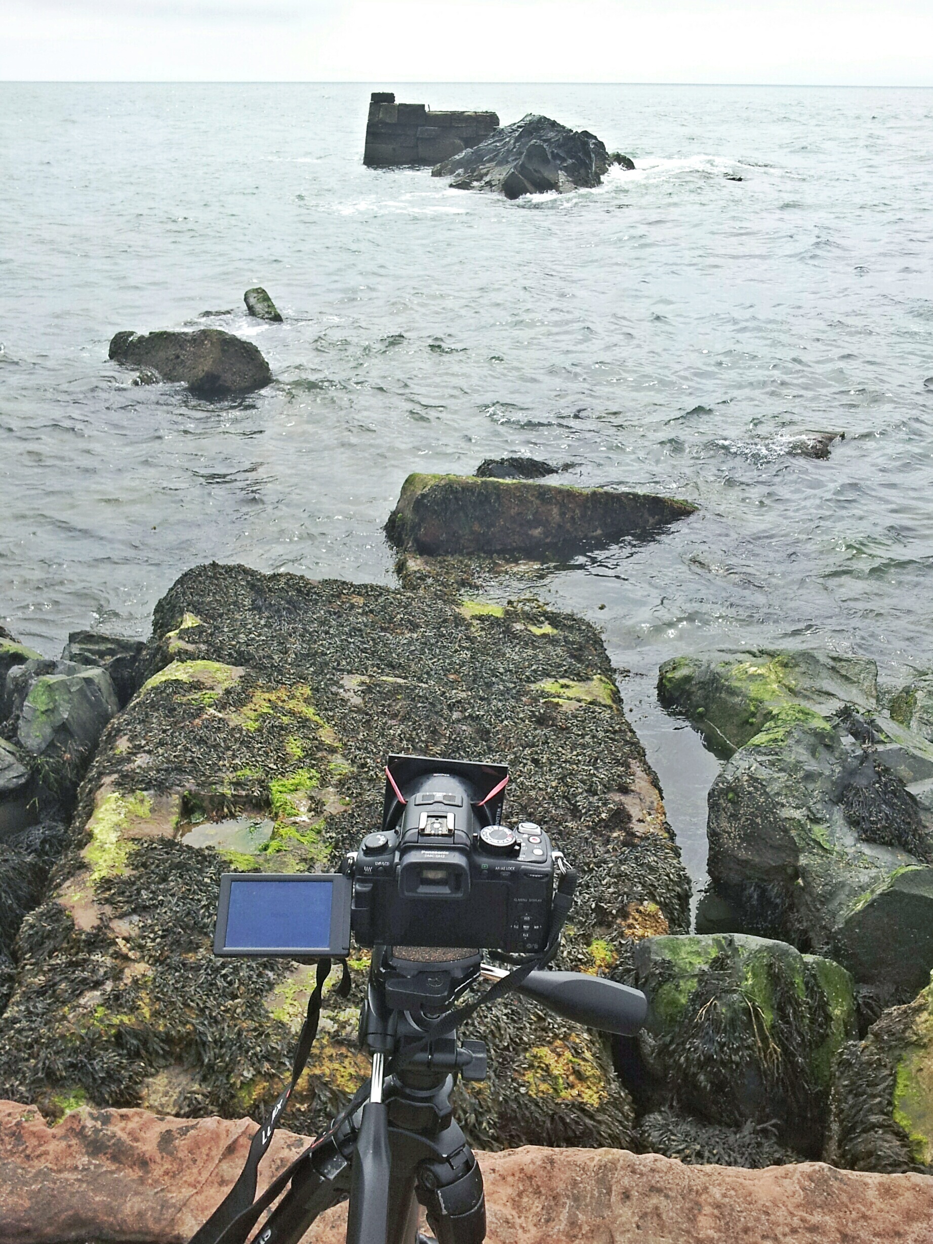
Decide which lenses, at which apertures, you want to profile. Make your own design, print it out at least A4 size, and affix it to a wall. We want the lighting to be as even as possible, so ideally use indoor artificial light after dark (ie this is a good project for a dark evening). Carefully, set up the camera on a tripod facing the chart square-on, and move close enough so the test-chart is just filling the frame.
Camera settings: use the lowest ISO setting possible (normally around 100), to minimize sensor noise. Use aperture-priority mode so it chooses the shutter-speed itself and fix the white-balance to counteract the indoor lighting. (For a daylight lightbulb, use daylight; otherwise, fluorescent or tungsten. Avoid auto-white-balance.)
Either use a remote-release cable or wireless trigger, or enable a 2-second self-timer mode to allow shaking to die down after pushing the shutter. Assuming the paper with the test-chart is still mostly white, use exposure-compensation (+2/3 EV).
For each lens and focal-length, start with the widest aperture and close-down by a third or half a stop, taking two photos at each aperture.
Open a small text-document and list each lens and focal-length in order as you go, along with any other salient features. (For example, with old manual prime lenses, note the start and final apertures and the interval size – may be half-stops, may be third of a stop.)
Use a RAW converter to process all the images identically: auto-exposure, fixed white-balance, and disable any sharpening, noise-reduction and rescaling you might ordinarily do. Output to 16-bit TIFF files.
Now, it is a given that a reasonable measure of pixel-level sharpness in an image, or part thereof, is its standard deviation. We can use the following Python script (requires numpy and OpenCV modules) to load image(s) and output the standard deviations of subsets of the images:
#!/usr/bin/env python

import sys, glob, cv, cv2
import numpy as np

def imageContrasts(fname):
  img = cv2.imread(fname, cv.CV_LOAD_IMAGE_GRAYSCALE)
  a=np.asarray(img)
  width=len(img[0])
  height=len(img[1])
  half=a[0:height//3, 0:width//3]
  corner=a[0:height//8, 0:width//8]
  return np.std(a), np.std(half), np.std(corner)

def main():
	files=sys.argv[1:]
	if len(files)==0:
		files=glob.glob("*.jpg")
	for f in files:
		co,cc,cf=imageContrasts(f)
		print "%s contrast %f %f %f" % (f, co, cc, cf)

if __name__=="__main__":
	main()
We can build a spreadsheet listing the files, their apertures and sharpnesses overall and in the corners, where vignetting typically occurs. We can easily make a CSV file by looping the above script and some exiftool magic across all the output TIFF files:
bash$ for f in *.tif
do
ap=$(exiftool $f |awk '/^Aperture/ {print $NF}' )
speed=$( exiftool $f |awk '/^Shutter Speed/ {print $NF}' )
conts=$(~/python/image-interpolation/image-sharpness-cv.py $f | sed 's/ /,/g')
echo $f,$ap,=$speed,$conts
done
Typical output might look like:
P1440770.tif,,=1/20,P1440770.tif,contrast,29.235214,29.918323,22.694936
P1440771.tif,,=1/20,P1440771.tif,contrast,29.253372,29.943765,22.739748
P1440772.tif,,=1/15,P1440772.tif,contrast,29.572350,30.566767,25.006098
P1440773.tif,,=1/15,P1440773.tif,contrast,29.513443,30.529055,24.942437
Note the extra `=’ signs; on opening this in LibreOffice Spreadsheet, the formulae will be evaluated and fractions converted to floating-point values in seconds instead. Remove the spurious `contrast’ column and add a header column (fname,aperture,speed,fname,overall,half,corner).
Analysis
Let’s draw some graphs. If you wish to stay with the spreadsheet, use a pivot table to average the half-image contrast values per aperture per lens and work off that. Alternatively, a bit of interactive R can lead to some very pretty graphs:
> install.package(ggplot2)
> library(ggplot2)
> data<-read.csv("sharpness.csv")
> aggs<-aggregate(cbind(speed,entire,third,corner) ~lens+aperture, data, FUN=mean)
> qplot(aggs$aperture, aggs$third, col=aggs$lens, data=aggs, asp=.5)+geom_smooth()
This will give a comparison of overall sharpness by aperture, grouped by lens. Typically we expect every lens to have a sweetspot aperture at which it is sharpest; my own examples are no exception: 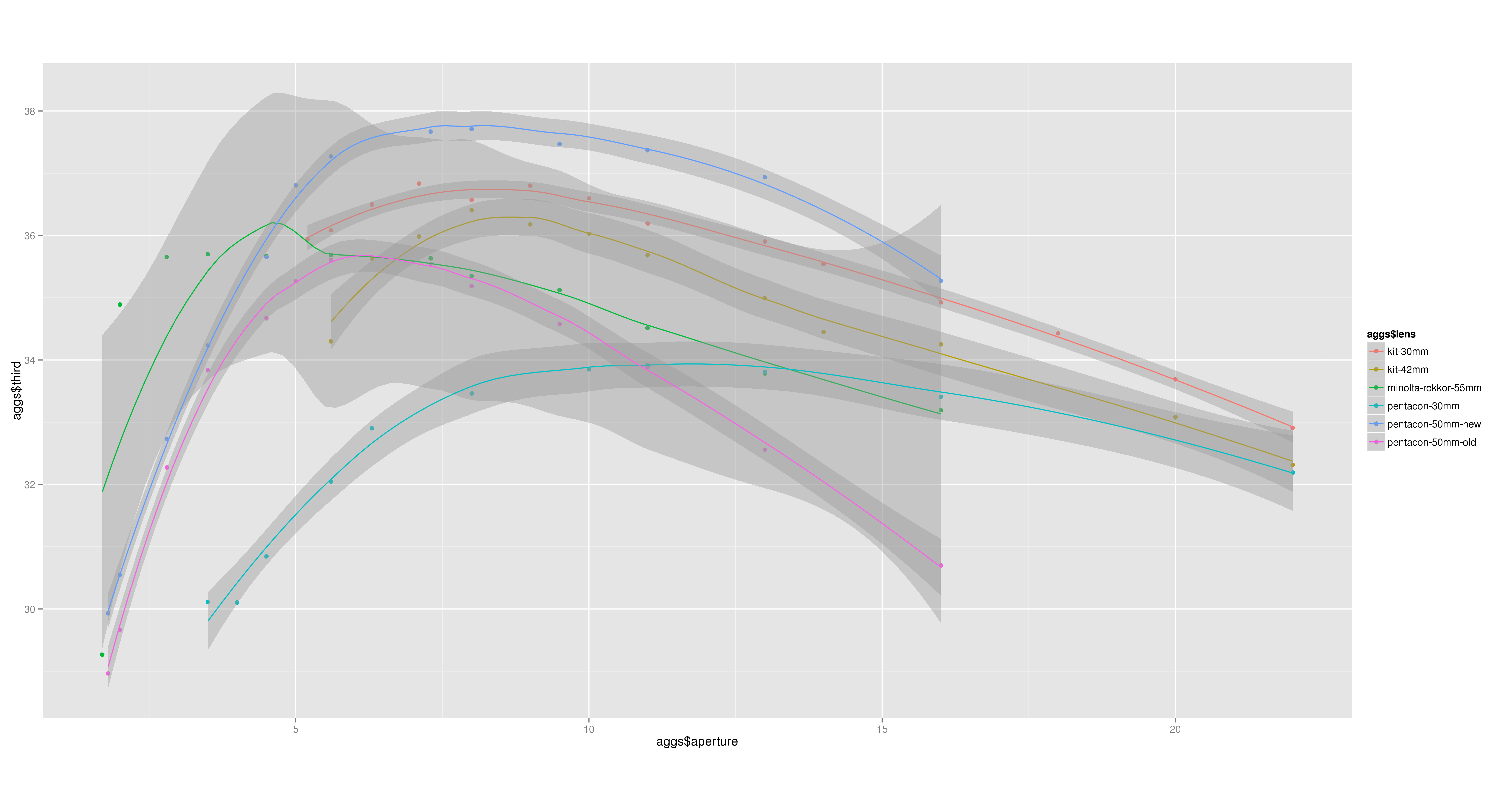 There are 5 lenses at play here: a kit 14-42mm zoom, measured at both 30mm and 42mm; a Minolta Rokkor 55mm prime; a Pentacon 30mm prime; and two Pentacon 50mm f/1.8 prime lenses, one brand new off eBay and one that’s been in the bag for 4 years.
The old Pentacon 50mm was sharpest at f/5.6 but is now the second-lowest at almost every aperture – we’ll come back to this. The new Pentacon 50mm is sharpest of all the lenses from f/5 onwards, peaking at around f/7.1. The kit zoom lens is obviously designed to be used around f/8; the Pentacon 30mm prime is ludicrously unsharp at all apertures – given a choice of kit zoom at 30mm or prime, it would have to be the unconventional choice every time. And the odd one out, the Rokkor 55mm, peaks at a mere f/4.
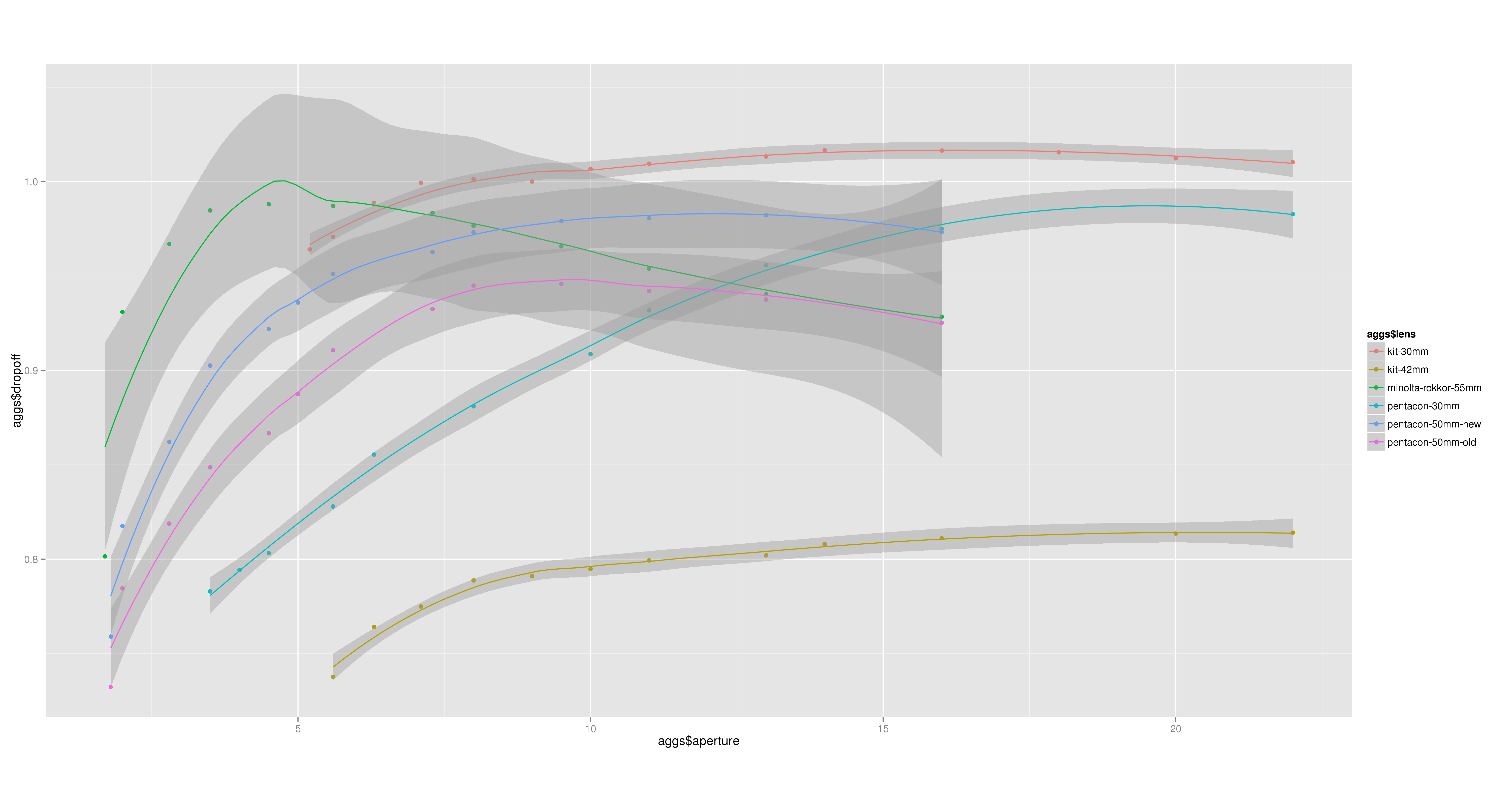
How about the drop-off, the factor by which the extreme corners are less sharp than the overall image? Again, a quick calculation and plot in R shows:
> aggs$dropoff < - aggs$corner / aggs$third
> qplot(aggs$aperture, aggs$dropoff, col=aggs$lens, data=aggs, asp=.5)+geom_smooth()
 Some observations:
- all the lenses show a similar pattern, worst vignetting at widest apertures, peaking somewhere in the middle and then attenuating slightly;
- there is a drastic difference between the kit zoom lens at 30mm (among the best performances) and 42mm (the worst, by far);
- the old Pentacon 50mm lens had best drop-off around f/8;
- the new Pentacon 50mm has least drop-of at around f/11;
- the Minolta Rokkor 55mm peaks at f/4 again.
So, why do the old and new Pentacon 50mm lenses differ so badly? Let’s conclude by examining the shutter-speeds; by allowing the camera to automate the exposure in aperture-priority mode, whilst keeping the scene and its illumination constant, we can plot a graph showing each lens’s transmission against aperture.
> qplot(aggs$aperture, log2(aggs$speed/min(aggs$speed)), col=aggs$lens, data=aggs, asp=.5)+geom_smooth()
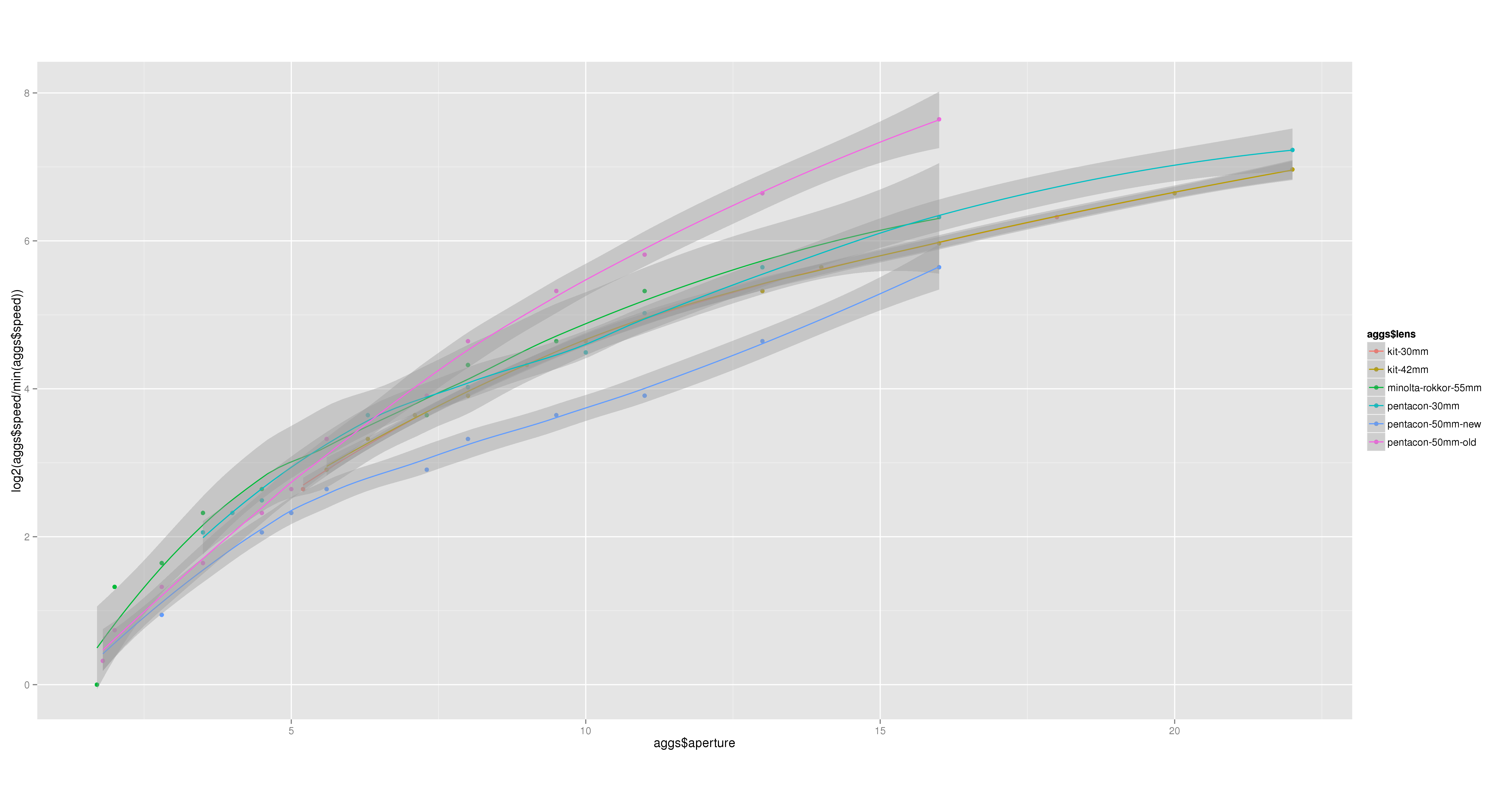 Here we see the new Pentacon 50mm lens seems to require the least increase in shutter-speed per stop aperture, while, above around f/7.1, the old Pentacon 50mm lens requires the greatest – rocketing off at a different gradient to everything else, such that by f/11 it’s fully 2 stops slower than its replacements.
There’s a reason for this: sadly, the anti-reflective coating is starting to come off in the centre of the front element of the old lens, in the form of a rough circle approximately 5mm diameter. At around f/10, the shutter iris itself is 5mm, so this artifact becomes a significant contributor to the overall exposure.
Conclusion
With the above data, informed choices can be made as to which lens and aperture suit particular scenes. When shooting a wide-angle landscape, I can use the kit zoom at f/8; for nature and woodland closeup work where the close-focussing distance allows, the Minolta Rokkor 55mm at f/4 is ideal.