A Geek in Lockdown

I’m comparatively fortunate that the coronavirus and covid-19 have not affected me or anyone I know directly. Having spent the last 15 years working from home, life has not changed as significantly as it has for others.

So, apart from staying home and doing nothing much, what’s a geek to do to contribute back?

First, contribute data. As often as I remember, I update the KCL/Zoe app to say I’m still alive.

Second, grid computing projects.

There’s a significant amount of computer power available and machines would otherwise spend their time idle. A couple of months before the coronavirus became known, I had already installed BOINC, perhaps the oldest and best-known grid-computing system. As the scale of the Covid-19 problem became more apparent, I discovered the Rosetta@Home project which has been working to predict structure of proteins involved in the disease.

For mobile devices, there is Vodafone’s DreamLab project which similarly uses one’s iphone/ipad/tablet’s downtime to perform computations hopefully to identify drugs to fight Covid-19.

Third, art.

This took a bit of thought, but recently RedBubble who I use for selling my photography added the option of selling masks alongside the usual prints, mugs, etc.

I wasn’t at all sure what to make of it. The idea of profiting off others’ health and necessity jarred with the idea of art being a luxury item. However, a friend pointed out that if face-masks are to become normalized in society, having interesting art designs on could make them more approachable. There’s also the bit where Redbubble match each mask bought with a donation to an appropriate charity. So, a net good thing then.

Inspiration struck and I spent much of the weekend designing an image to represent the coronavirus (using a fragment of its gene sequence as a background, naturally) and even rendering a little video from it, both using Povray, my favoured ray-tracing software from the late 1990s(!). Naturally I made the scene description and other sources available as open-source: the-lurgy (on github).

The “lurgy” design and a selection of other landscape images are available on redbubble as face-masks with a profit margin set to 0.

And of course work continues, producing more photos to go on my website, ShinyPhoto

ShinyPhoto: New Website

The old ShinyPhoto website was getting a bit long in the tooth. It saw several versions of Python come and go and increasingly suffered from bitrot. (Notably, a mutual incompatibility in the CGI module between python versions; it ran for so long the backend storage engine I used became deprecated with no easy way out but to revert to one I wrote myself – not a good reason to rely on third-party libraries!)

So, for the past couple of months I’ve been learning my way around Javascript and node.js and have replaced the site with a new gallery to show-off my photos.

Being me, it’s a bit geeky. With web-design there are so many angles to consider, but here are a few aspects that stick in the mind:

Technical: no XSLT; this is the first time in nearly 20 years where I’ve used a different templating language – in this case, Mustache since it does need to be able to produce non-HTML data as well.

Learning: there’s a whole ecosystem of node.js packages (NPMs) that have come in handy, from the Express webserver to image-resizing utilities (some of which are faster than others!).

Data: in my more professional work capacity I deal with data-storage on a daily basis, so it has some passing interest. One of the problems with the old site was its inability to extract metadata from images; because this instance’s primary focus is the organization and display of photos, I decided that the JPEG should contain all the data displayed – title, description, geotagging, keywords all extracted from one upload and the less manual editing effort required, the better. Essentially, digiKam is both organizer and implicit website editor on my desktop.

Database: with the unit of data being the JPEG, presented as a page per photo, that maps well into a document-oriented model such as one of the NoSQL JSON-based databases. Unfortunately MongoDB disgraced themselves by choosing a non-open-source licence recently, so I was pleased to discover CouchDB – a modular system sharing protocols (JSON-over-HTTP(S)) and query language (MangoDB) across different storage backends with the advantage that I can start from the PouchDB pure node.js implementation but switch to an external version of the same with a quick data-replication later if need be. So far, it’s coping fine with 1.1GB of JPEG data (stored internally as attachments) and 70MB of log data.

Configurability: several aspects of the site are configurable, from the internal and external navigation menus to the cache-validity/timeout on images.

Scalable: my initial thought was to keep image-resizing pure-javascript and rely on nginx caching for speed; however, that would lose the ability to count JPEG impressions (especially thumbnails), so I switched to a mixed JS/C NPM and now resizing is sufficiently fast to run live. The actual node.js code itself also runs cleanly – feels very snappy in the browser after the old python implementation.

Metadata/SEO: the change of templating engine has meant specific templates can be applied to specific kinds of pages, rather than imposing one structure across the whole site; different OpenGraph and Twitter-Card metadata applies on the homepage, gallery and individual photo pages.

Statistics: lots of statistics. There are at least three aspects where statistics rule:

  • the usual analytics; it’s always handy to keep an eye on the most-popular images, external referrers, etc. The site uses its own application-level logging to register events on the page-impression scale, so the log data is queryable without having to dig through CLF webserver logs.
  • how should a photo gallery be sorted? By popularity, by date? Do thumbnails count? What about click-through rate? The new site combines all three metrics to devise its own score-function which is recalculated across all images nightly and forms the basis of a display order. (It surprises me that there are photo-galleries that expect people to choose the sort order by hand, or even present no obvious order at all.)
  • how should a photo-gallery be organized? My work is very varied, from bright colour to black and white, from sky to tree to mountain and water, from fast to long exposure, from one corner of the country to another, as the landscape leads; I did not want to impose a structure only to have to maintain it down the line. Accordingly, the new ShinyPhoto is self-organizing: within any slice through the gallery, a set of navigation tags is chosen that splits the images closest to half. Relatedly, the images on the homepage used to be a static selection, manually edited; now they are chosen dynamically by aspect-ratio and score.
  • Marketing: some aspects of the layout now enjoy a/b testing – no cookies required, but another hash function determines the site appearance and I can check which work best over time.

So far, it’s proving pleasantly easy to live with; apart from the continual debugging and adding of new features – fortunately now slowing down – I’m adding photos at a rate of a handful a day both to the site and to a new RedBubble account in case anyone wants to buy them, one way or another.

So apparently I now like the whole node.js ecosystem. It’s blown away the cobwebs of running – or more accurately not-running – a legacy website, whilst retaining full control of the appearance and structure of the site not handing that over to some third-party site designer.

A good way to start a new year, methinks.

Focus-Stacking with the Fuji X-H1

For years I’ve been a fan of superresolution – taking multiple images of a scene with subtle sub-pixel shifts and upscaling before blending to give a greater resolution photo than any one source.

One of the features I used occasionally on the Pentax K-1 was its pixel-shift, whereby the sensor moved four times around a 1px square; this gives an improved pixel-level resolution and full chroma detail at each point.

Having exchanged that for the Fuji X-H1, I still look to perform super-resolution one way or another. Hand-held HDR always works – in this case even better than either the K-1 or the X-T20 because the X-H1 permits 5 or 7 frames per bracket at ±2/3EV each, which is ideal.

But I thought I’d experiment with a different approach: focus-stacking. This way, the camera racks the focus from foreground to background in many fine steps. Keeping the focal-length the same, the effective zoom changes subtly between successive images. Essentially, where hand-held HDR varies the position stochastically in an X-Y plane, focus-stacking means pixels from the source frames track a predictable radial line in the superresolved image.

The X-H1 has focus-bracketing but leaves the blending up to the user in post. That’s OK.

First, an overview of the scene:

Scene overview: Fuji X-H1, 18-135mm lens at 127mm, f/8 narrow DoF

The X-H1 made 50 frames, focussing progressively from front to back. These were blended using enfuse:

time align_image_stack -a /tmp/aligned_ -d -i -x -y -z -C [A-Z]*.{tif,tiff,jpg,JPG,png}
time enfuse -o "fused_$base" /tmp/aligned_* -d 16 -l 29 --hard-mask --saturation-weight=0 --entropy-weight=0.4 --contrast-weight=1 --exposure-weight=0 --gray-projector=l-star --contrast-edge-scale=0.3

The results are a little strange to behold – while the effective DoF is much increased (the distant wood texture is clear) the rock detail is quite soft; I suspect some of the above numbers need tweaking.

However, with a bit of work – both enhancing the local contrast and using in-painting to tidy up the rock itself – a pleasant image emerges:

The final polished result: banded rock on wood, Fuji X-H1

A definite improvement. I may have to use it in my landscape work a bit 🙂

How Many Megapixels?

There are several cliches in the field of megapixel-count and resolution required for acceptable photographic prints.

In no particular order:

  • 300dpi is “fine art”
  • you don’t need as many dpi for larger prints because typically they’re viewed further away
  • my printer claims to do 360dpi or 1440dpi or …
  • 24 megapixels is more than enough for anything
  • “for a 5″ print you need 300-800pixels, for medium to large calendars 800-1600 pixels, for A4 900-1600px, for an A3 poster 1200 to 2000px, for an A2 poster 1500 to 2400px, …” (taken from a well-known photo-prints website guidelines)
  • it’s not about the megapixels it’s about the dynamic range

There are probably more set arguments in the field, but all are vague, arising from idle pontificating and anecdote over the last couple of centuries.

Here’s a key question: in a list of required image resolutions by print size, why does the number of dpi required drop-off with print size? What is the driving factor and might there be an upper bound on the number of megapixels required to make a print of any size?

We can flip this around and say that if prints are expected to be viewed at a distance related to their size, then it is no longer a matter of absolute measurements in various dimensions but rather about how much field of view they cover. This makes it not about the print at all, but about the human eye, its field of view and angular acuity – and the numbers are remarkably simple.

From wikipedia, the human eye’s field of view is 180-200 degrees horizontally by 135 degrees vertically (ie somewhere between 4:3 and 3:2 aspect-ratios).  Its angular acuity is between 0.02 to 0.03 deg.

If we simply divide these numbers we end up with a number of pixels that the eye could resolve.

At one end of the range,

 180*135 /0.03 / 0.03 / 1024 / 1024 = 25.75 (6000 x 4500)

and at the other:

200*135 / 0.02 / 0.02 / 1024 / 1024 = 64.37 (10,000 x 6750)

In the middle,

180*135 / 0.025 / 0.025 / 1024 / 1024 = 37.1 (7200 x  5400)

Significant points:

  • this is no longer about absolute print sizes; it’s simply about being able to view a print without one’s eye perceiving pixellation
  • the numbers correlate reassuringly with numbers of megapixels seen in real-world dSLR sensors today
  • you can reasonably say that if you have 64 Megapixels then you can make a print of any size from it
  • you can make an image with more than 64 megapixels if you want to, but the reasons for doing so are not directly to do with resolution – they might be
    in order that you can  crop it – either to physically crop the image in post-processing or to view it from a closer distance than that required merely to fill your eyes’ field of view
    or maybe for pixel-binning to reduce noise, give smoother tonality, etc
  • 24 megapixels is not enough for much; rather it’s is a turning-point: the bare minimum number of pixels for a person of limited acuity to resolve assuming they slightly less than fill their field of view with the print. 36MPel is more usable and 64 will keep you in business selling fine quality wall art.

Now we know how many megapixels are required for various real-world purposes, all that matters is making them good megapixels. Physics to the rescue.


Trying something a little different

For years now, my photo-processing workflow has been 100% open-source. However, in the interests of greater portability – hack on photos whilst on the go – and partly gratuitously for the sake of variety, I recently acquired an iPad Pro 10.5″ and installed the Affinity Photo app.

As a user experience goes, it’s really quite pleasant. The best way to synchronise files around the LAN seems to be Seafile, which is open-source and available for Linux, iOS and android. My Linux-based workflow regularly produces 64-megapixel images, working on multiple intermediate TIFF files, 16-bit ProPhotoRGB-linear; somewhat surprisingly, seafile, the iPad and Affinity Photo seem able to handle files around 450MiB in size. There are a few small gotchas – I had to import a few ICC colour profiles by hand and as yet, there doesn’t seem to be a way to customise export options (so you have to select JPEG 99% sRGB lanczos yourself afresh every time); I’m sure these things will come in time however.

So here’s a shot from last Sunday afternoon. As I was heading out of Muthill I saw this characterful old tree in a field; on the return journey a few hours later, not only was it still there but the clouds were darker in the background and the golden sunlight caught the bare branches. A very quick bit of parking and even quicker sprint back to the optimum viewpoint and it looked stunning. So I processed it a little further, realising an intention for how it should look that was apparent from the start.

Sunlit tree

Pentax K-1: an open-source photo-processing workflow

There is a trope that photography involves taking a single RAW image, hunching over the desktop poking sliders in Lightroom, and publishing one JPEG; if you want less noise you buy noise-reduction software; if you want larger images, you buy upscaling software. It’s not the way I work.

I prefer to make the most of the scene, capturing lots of real-world photons as a form of future-proofing. Hence I was pleased to be able to fulfil a print order last year that involved making a 34″-wide print from an image captured on an ancient Lumix GH2 many years ago. Accordingly, I’ve been blending multiple source images per output, simply varying one or two dimensions: simple stacking, stacking with sub-pixel super-resolution, HDR, panoramas and occasionally focus-stacking as the situation demands.

I do have a favoured approach, which is to compose the scene as closely as possible to the desired image, then shoot hand-held with HDR bracketing; this combines greater dynamic range, some noise-reduction and scope for super-resolution (upscaling).

I have also almost perfected a purely open-source workflow on Linux with scope for lots of automation – the only areas of manual intervention were setting the initial RAW conversion profile in RawTherapee and the collation of images into groups in order to run blending in batch.

After a while, inevitably, it was simply becoming too computationally intensive to be upscaling and blending images in post, so I bought an Olympus Pen-F with a view to using its high-resolution mode, pushing the sub-pixel realignment into hardware. That worked, and I could enjoy two custom setting presets (one for HDR and allowing walk-around shooting with upscaling, one for hi-res mode on a tripod), albeit with some limitations – no more than 8s base exposure (hence exposure times being quoted as “8x8s”), no smaller than f/8, no greater than ISO 1600. For landscape, this is not always ideal – what if 64s long exposure doesn’t give adequate cloud blur, or falls between one’s ND64 little- and ND1000 big-stopper filters? What if the focal length and subject distance require f/10 for DoF?

All that changed when I swapped all the Olympus gear for a Pentax K-1 a couple of weekends ago. Full-frame with beautiful tonality – smooth gradation and no noise. A quick test in the shop and I could enable both HDR and pixel-shift mode and save RAW files (.PEF or .DNG) and in the case of pixel-shift mode, was limited to 30s rather than 8s – no worse than regular manual mode before switching to bulb timing. And 36 megapixels for both single and multi-shot modes. Done deal.

One problem: I spent the first evening collecting data, er, taking photos at a well-known landscape scene, came home with a mixture of RAW files, some of which were 40-odd MB, some 130-odd MB; so obviously multiple frames’ data was being stored. However, using RawTherapee to open the images – either PEF or DNG – it didn’t seem like the exposures were as long as I expected from the JPEGs.

A lot of reviews of the K-1 concentrate on pixel-shift mode, saying how it has options to correct subject-motion or not, etc, and agonizing over how which commercial RAW-converter handles the motion. What they do not make clear is that the K-1 only performs any blend when outputting JPEGs, which is also used as the preview image embedded in the RAW file; the DNG or PEF files are simply concatenations of sub-frames with no processing applied in-camera.

On a simple test using pixel-shift mode with the camera pointing at the floor for the first two frames and to the ceiling for the latter two, it quickly becomes apparent that RawTherapee is only reading the first frame within a PEF or DNG file and ignoring the rest.

Disaster? End of the world? I think not.

If you use dcraw to probe the source files, you see things like:

zsh, rhyolite 12:43AM 20170204/ % dcraw -i -v IMGP0020.PEF

Filename: IMGP0020.PEF
Timestamp: Sat Feb  4 12:32:52 2017
Camera: Pentax K-1
ISO speed: 100
Shutter: 30.0 sec
Aperture: f/7.1
Focal length: 31.0 mm
Embedded ICC profile: no
Number of raw images: 4
Thumb size:  7360 x 4912
Full size:   7392 x 4950
Image size:  7392 x 4950
Output size: 7392 x 4950
Raw colors: 3
Filter pattern: RG/GB
Daylight multipliers: 1.000000 1.000000 1.000000
Camera multipliers: 18368.000000 8192.000000 12512.000000 8192.000000

On further inspection, both PEF and DNG formats are capable of storing multiple sub-frames.

After a bit of investigation, I came up with an optimal set of parameters to dcraw with which to extract all four images with predictable filenames, making the most of the image quality available:

dcraw -w +M -H 0 -o /usr/share/argyllcms/ref/ProPhotoLin.icm -p "/usr/share/rawtherapee/iccprofiles/input/Pentax K200D.icc" -j -W -s all -6 -T -q 2 -4 "$filename"

Explanation:

  • -w = use camera white-balance
  • +M = use the embedded colour matrix if possible
  • -H 0 = leave the highlights clipped, no rebuilding or blending
    (if I want to handle highlights, I’ll shoot HDR at the scene)
  • -o = use ProPhotoRGB-linear output profile
  • -p = use RawTherapee’s nearest input profile for the sensor (in this case, the K200D)
  • -j = don’t stretch or rotate pixels
  • -W = don’t automatically brighten the image
  • -s all = output all sub-frames
  • -6 = 16-bit output
  • -T = TIFF instead of PPM
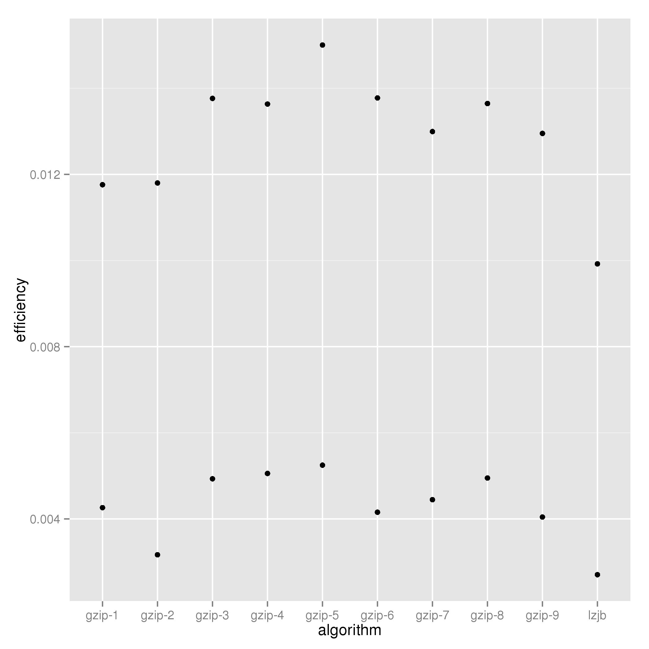
  • -q 2 = use the PPG demosaicing algorithm
    (I compared all 4 options and this gave the biggest JPEG = hardest to compress = most image data)
  • -4 = Lienar 16-bit

At this point, I could hook in to the workflow I was using previously, but instead of worrying how to regroup multiple RAWs into one output, the camera has done that already and all we need do is retain the base filename whilst blending.

After a few hours’ hacking, I came up with this little zsh shell function that completely automates the RAW conversion process:

pic.2.raw () {
        for i in *.PEF *.DNG
        do
                echo "Converting $i"
                base="$i:r" 
                dcraw -w +M -H 0 -o /usr/share/argyllcms/ref/ProPhotoLin.icm -p "/usr/share/rawtherapee/iccprofiles/input/Pentax K200D.icc" -j -W -s all -6 -T -q 2 -4 "$i"
                mkdir -p converted
                exiftool -overwrite_original_in_place -tagsfromfile "$i" ${base}.tiff
                exiftool -overwrite_original_in_place -tagsfromfile "$i" ${base}_0.tiff
                mv ${base}.tiff converted 2> /dev/null
                mkdir -p coll-$base coll-$base-large
                echo "Upscaling"
                for f in ${base}_*.tiff
                do
                        convert -scale "133%" -sharpen 1.25x0.75 $f coll-${base}-large/${f:r}-large.tiff
                        exiftool -overwrite_original_in_place -tagsfromfile "$i" coll-${base}-large/${f:r}-large.tiff
                done
                mv ${base}_*tiff coll-$base 2> /dev/null
        done
        echo "Blending each directory"
        for i in coll-*
        do
          (cd $i && align_image_stack -a "temp_$i_" *.tif? && enfuse -o "fused_$i.tiff" temp_$base_*.tif \
           -d 16 \
           --saturation-weight=0.1 --entropy-weight=1 \
           --contrast-weight=0.1 --exposure-weight=1)
        done
        echo "Preparing processed versions"
        mkdir processed
        (
                cd processed && ln -s ../coll*/f*f . && ln -s ../converted/*f .
        )
        echo "All done"
}

Here’s how the results are organized:

  • we start from a directory with source PEF and/or DNG RAW files in it
  • for each RAW file found, we take the filename stem and call it $base
  • each RAW is converted into two directories, coll-$base/ consisting of the TIFF files and fused_$base.tiff, the results of aligning and enfuse-ing
  • for each coll-$base there is a corresponding coll-$base-large/ with all the TIFF images upscaled 1.33 (linear) times before align+enfusing
    This gives the perfect blend of super-resolution and HDR when shooting hand-held
    The sharpening coefficients given to ImageMagick’s convert(1) command have been chosen from a grid comparison; again the JPEG conversion is one of the largest showing greatest image detail.
  • In the case of RAW files only containing one frame, it is moved into converted/ instead for identification
  • All the processed outptus (single and fused) are collated into a ./processed/ subdirectory
  • EXIF data is explicitly maintained at all times.

The result is a directory of processed results with all the RAW conversion performed using consistent parameters (in particular, white-balance and exposure come entirely from the camera only) so, apart from correcting for lens aberrations, anything else is an artistic decision not a technical one. Point darktable at the processed/ directory and off you go.

All worries about how well “the camera” or “the RAW converter” handle motion in the subject in pixel-shift mode are irrelevant when you take explicit control over it yourself using enfuse.

Happy Conclusion: whether I’m shooting single frames in a social setting, or walking around doing hand-held HDR, or taking my time to use a tripod out in the landscape (each situation being a user preset on the camera), the same one command suffices to produce optimal RAW conversions.


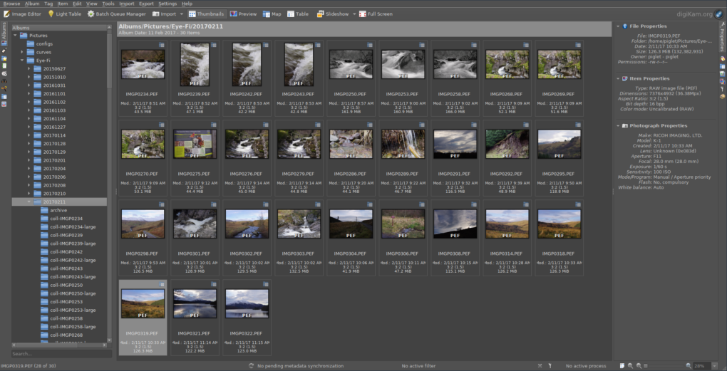
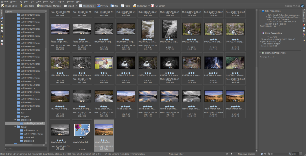
digiKam showing a directory of K-1 RAW files ready to be converted

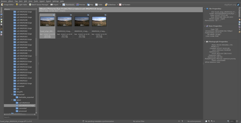
One of the intermediate directories, showing 1.33x upscaling and HDR blending

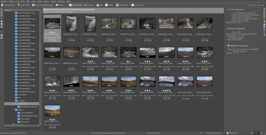
Results of converting all RAW files – now just add art!

The results of running darktable on all the processed TIFFs – custom profiles applied, some images converted to black+white, etc

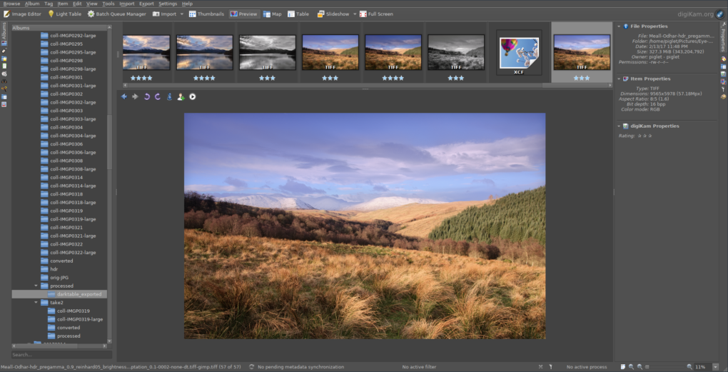
One image was particularly outstanding so has been processed through LuminanceHDR and the Gimp as well

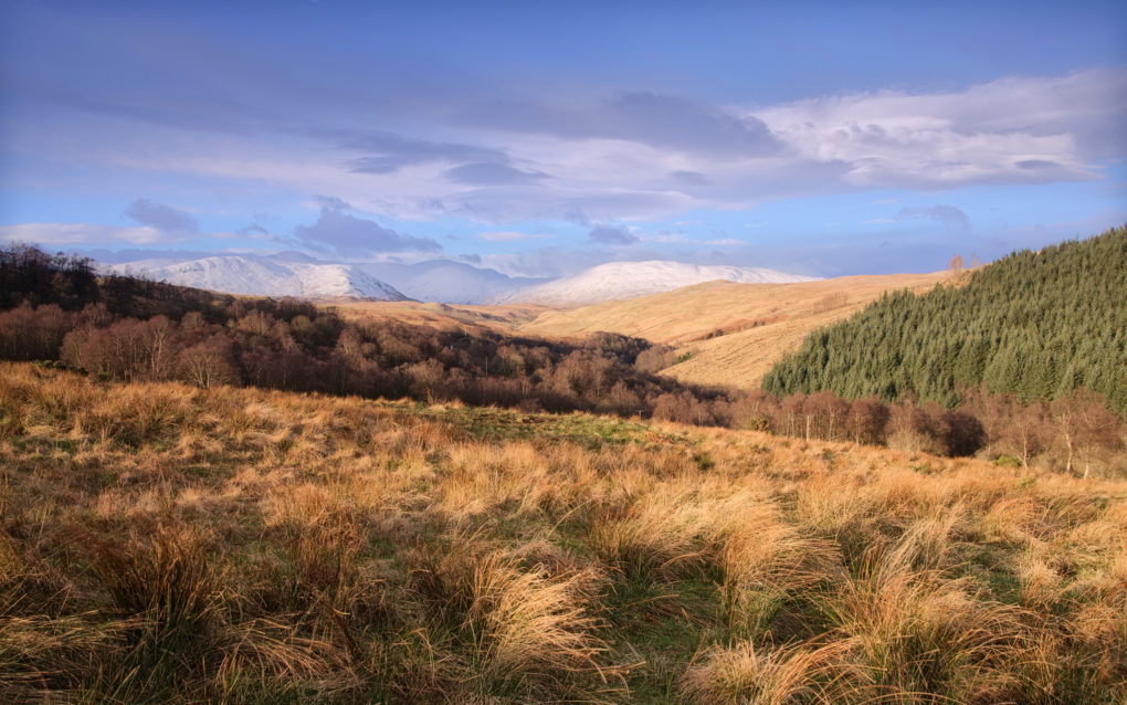
Meall Odhar from the Brackland Glen, Callander

Announcing Timelapse.jl – frame interpolation for timelapse photography

A few years ago I wrote a python utility for interpolating a greater number of frames from a smaller set, for use in timelapse video/photography.

Recently, I’ve been trying to learn Julia. As a small challenge – to fulfil a potential forthcoming need – and because it claimed to be quite a fast language – I’ve rewritten the core of the script.

It’s quite refreshing – none of the gratuitous OO classes I had to create with Python, just a couple of functions to do the essential interpolation. And watching the output frames flash by… it’s pretty nippy, too.

It doesn’t yet support EXIF directly, nor can it modify images directly on the fly, but if you want to have a play then go download it from Githubhttps://github.com/spodzone/Timelapse.jl

Determining the best ZFS compression algorithm for email

I’m in the process of setting up a FreeBSD jail in which to run a local mail-server, mostly for work. As the main purpose will be simply archiving mails for posterity (does anyone ever actually delete emails these days?), I thought I’d investigate which of ZFS’s compression algorithms offers the best trade-off between speed and compression-ratio achieved.

The Dataset

The email corpus comprises 273,273 files totalling 2.14GB; individually the mean size is 8KB, the median is 1.7KB and the vast majority are around 2.5KB.

The Test

The test is simple: the algorithms consist of 9 levels of gzip compression plus a new method, lzjb, which is noted for being fast, if not compressing particularly effectively.

A test run consists of two parts: copying the entire email corpus from the regular directory to a new temporary zfs filesystem, first using a single thread and then using two parallel threads – using the old but efficient   find . | cpio -pdv   construct allows spawning of two background jobs copying the files sorted into ascending and descending order – two writers, working in opposite directions. Because the server was running with a live load at the time, a test was run 5 times per algorithm – a total of 13 hours.

The test script is as follows:

#!/bin/zsh

cd /data/mail || exit -1

zfs destroy data/temp

foreach i ( gzip-1 gzip-2 gzip-3 gzip-4 gzip-5 gzip-6 \
	gzip-7 gzip-8 gzip-9 lzjb ) {
  echo "DEBUG: Doing $i"
  zfs create -ocompression=$i data/temp
  echo "DEBUG: Partition created"
  t1=$(date +%s)
  find . | cpio -pdu /data/temp 2>/dev/null
  t2=$(date +%s)
  size=$(zfs list -H data/temp)
  compr=$(zfs get -H compressratio data/temp)
  echo "$i,$size,$compr,$t1,$t2,1"
  zfs destroy data/temp

  sync
  sleep 5
  sync

  echo "DEBUG: Doing $i - parallel"
  zfs create -ocompression=$i data/temp
  echo "DEBUG: Partition created"
  t1=$(date +%s)
  find . | sort | cpio -pdu /data/temp 2>/dev/null &
  find . | sort -r | cpio -pdu /data/temp 2>/dev/null &
  wait
  t2=$(date +%s)
  size=$(zfs list -H data/temp)
  compr=$(zfs get -H compressratio data/temp)
  echo "$i,$size,$compr,$t1,$t2,2"
  zfs destroy data/temp
}

zfs destroy data/temp

echo "DONE"

Results

The script’s output was massaged with a bit of commandline awk and sed and vi to make a CSV file, which was loaded into R.

The runs were aggregated according to algorithm and whether one or two threads were used, by taking the mean removing 10% outliers.

Since it is desirable for an algorithm both to compress well and not take much time to do it, it was decided to define efficiency = compressratio / timetaken.

The aggregated data looks like this:

algorithm nowriters eff timetaken compressratio
1 gzip-1 1 0.011760128 260.0 2.583
2 gzip-2 1 0.011800408 286.2 2.613
3 gzip-3 1 0.013763665 196.4 2.639
4 gzip-4 1 0.013632926 205.0 2.697
5 gzip-5 1 0.015003015 183.4 2.723
6 gzip-6 1 0.013774746 201.4 2.743
7 gzip-7 1 0.012994211 214.6 2.747
8 gzip-8 1 0.013645055 203.6 2.757
9 gzip-9 1 0.012950727 215.2 2.755
10 lzjb 1 0.009921776 181.6 1.669
11 gzip-1 2 0.004261760 677.6 2.577
12 gzip-2 2 0.003167507 1178.4 2.601
13 gzip-3 2 0.004932052 539.4 2.625
14 gzip-4 2 0.005056057 539.6 2.691
15 gzip-5 2 0.005248420 528.6 2.721
16 gzip-6 2 0.004156005 709.8 2.731
17 gzip-7 2 0.004446555 644.8 2.739
18 gzip-8 2 0.004949638 566.0 2.741
19 gzip-9 2 0.004044351 727.6 2.747
20 lzjb 2 0.002705393 900.8 1.657

A plot of efficiency against algorithm shows two clear bands, for the number of jobs writing simultaneously.

Analysis

In both cases, the lzjb algorithm’s apparent speed is more than compensated for by its limited compression ratio achievements.

The consequences of using two writer processes are two-fold: first, the overall efficiency is not only halved, but it’s nearer to only a third that of the single writer – there could be environmental factors at play such as caching and disk i/o bandwidth. Second, the variance overall has increased by 8%:

> aggregate(eff ~ nowriters, data, FUN=function(x) { sd(x)/mean(x, trim=0.1)*100.} )
 nowriters eff
1 1 21.56343
2 2 29.74183

so choosing the right algorithm has become more significant – and it remains gzip-5 with levels 4, 3 and 8 becoming closer contenders but gzip-2 and -9 are much worse choices.

Of course, your mileage may vary; feel free to perform similar tests on your own setup, but I know which method I’ll be using on my new mail server.

Definitions of Geek Antiquity

I can see already that this will probably be a series of more than one post…

You know you’ve been a geek a while when you find files like these lying around:

 -rw-r--r-- 1 tim users 16650 Apr 24 2001 .pinerc
...
D drwxr-xr-x 3 tim users   76 Aug 18 2003 .sawfish
  -rw------- 1 tim users  324 Jan 14 2003 .sawfishrc
D drwxr-xr-x 3 tim users   95 Apr 24 2001 .sawmill
  -rw-r--r-- 1 tim users 4419 Apr 24 2001 .sawmillrc

Just in case there’s any doubt: I used Pine from about 1995 to 2000, before I bypassed mutt in favour of Emacs and Gnus. Sawmill was the original name before Sawfish renamed itself; either way, I no longer use just a simple window-manager but the whole KDE environment.

A slight tidy-up is called for…

Old is the new… old, really

Time for a bit of a rant, geek-style.

For about 15 months I’ve used a Samsung Galaxy Note as mobile phone of choice. And truth be told, I’ve hated all bar the first 10 minutes of it. The lack of RAM has made me reconsider what apps I use, favouring Seesmic for combined Facebook+Twitter over separate apps; it still makes it horrendously slow for running anything interactive – as an example, by the time I’d got the thing unlocked and fired-up HDR Camera+, a rainbow had entirely gone! Spontaneity, we do not have it.

What they don’t tell you is that the leverage available when coupling these large screens with tiny thin USB connectors is a recipe for disaster. I’ve bent the pins on more cables than I care to think, trying to wiggle the thing for optimum solid connectivity; just before Christmas last year it finally died and the internal USB connector broke, requiring a repair under warranty – the first time I’ve ever had to send back a phone to be fixed.

Anyway, yesterday evening it threw a hissy-fit and spontaneously discharged the battery all the way down to empty, despite being plugged in (and, given that the wiggly-connector issues seemed to be returning, I made doubly sure that the power icon said charging). I recharged the battery overnight with the phone turned off, and yet this morning it still refused to boot up. It did something like this a while ago, and leaving it overnight was sufficient to reset itself; today, it’s had all day and still isn’t powering on any more.

So this morning I dug out my old HTC Hero, the first Android phone I ever used, and flashed it with CyanogenMod and updated the radio package. After a bit lot of faffing around, hunting and installing SSL root CA certificates to allow it to talk to Google and rebooting, I’m now powered by a custom ROM and sufficiently uptodate that Google Talk has been replaced by Hangouts. Yay, geek-cred!

The Samsung problem might be as simple as a dead battery; however, after the Christmas fiasco I really can’t be bothered trying to fix it any more and will look forward to getting something better later in the year.

Unfortunately it means a few changes on this blog; the camera is down from 8 megapixels to 5MPel and I won’t be shooting with HDR Camera+ or processing images on the phone with Aviary any more. Still, it does work for capturing the odd image and I can achieve some suitably strange processing effects on the notebook with darktable if I want.

Meanwhile I’m back getting my communication and maps on the go again. And the Hero is living up to its name.